
ERDC/CHL CETN-IV-27
September 2000
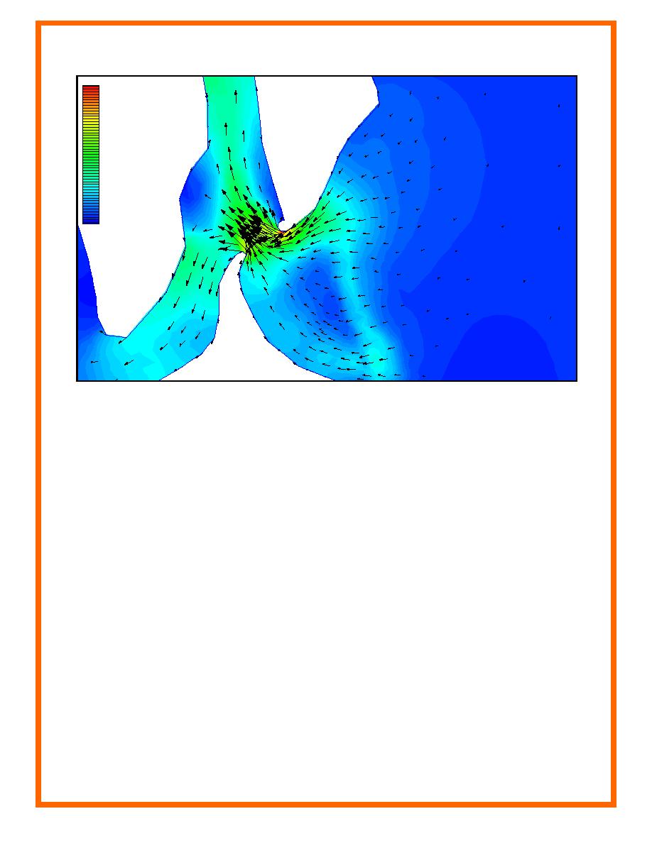
velocity mag 1 : 18.500
6.86
6.30
5.74
5.18
4.62
4.06
3.50
2.94
2.38
1.82
1.26
0.70
0.14
Figure 5. An isovel-filled contour plot with velocity vector overlay (units in ft/s) that provides quantitative
information over the entire area of interest (Velocity is in feet per second. To convert to meters per
second, multiply by 0.3048)
Finally, in Figure 6, the logic behind Figure 5 extends one step further. In this figure, contours of
change in velocity are shown with increased velocities in red and decreased velocities in blue.
These types of formats are particularly helpful for the evaluation of proposed or expected
changes in bathymetry, channel alignment, or structural modifications. To generate this type of
plot, the hydrodynamic model must be run twice -- once for baseline conditions and once for the
changed conditions under consideration. Computed velocity values for each model simulation
are then overlaid to create a single new output file representing the change in velocity at each
element. These data are then displayed, as in the contours shown in Figure 6. The color contours
readily highlight those areas which may become prone to erosion (red) and deposition (blue)
should the condition change. This CETN provides guidelines for creating plots from
hydrodynamic output, such as Figures 4 through 6, that improve the transfer of flow information,
enable an improved level of understanding about the model results, and provide insight into
sediment transport without having to run a time-dependent sediment transport model.
Although this CETN functions together with the DMS as a guide for identifying areas of
persistent shoaling through graphical interpretation, the methods described herein are applicable
for displaying hydrodynamic output of any kind, including those obtained from physical models.
This CETN first reviews the platform (SMS) (Brigham Young University 1999) for creating the
types of plot presented in Figures 4 through 6, and then discusses presentation of the direct
hydrodynamic output. Finally, the discussion ends with methods to manipulate the output to
gain further insight into the flow physics and sediment transport.
4

 Previous Page
