
ERDC/CHL CHETN-I-64
September 2001
STWAVE solves the steady-state conservation of spectral wave action along backward traced
wave rays (Jonsson 1990) with the source/sink terms of surf-zone wave breaking, wind input,
wave-wave interaction, and whitecapping (Resio 1987, 1988a, 1988b; Smith, Sherlock, and
Resio 2001). The STWAVE governing equations are numerically solved using finite-difference
methods on a Cartesian grid. Model grid cells are square. STWAVE operates in a local
coordinate system, with the x-axis oriented in the cross-shore direction and the y-axis oriented
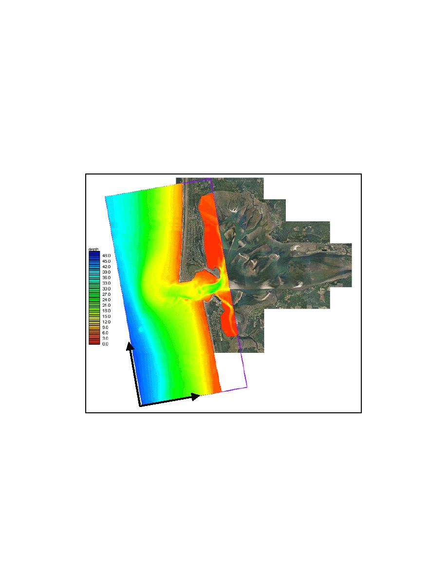
along the shore. Figure 2 shows an example STWAVE bathymetry grid for Grays Harbor,
Washington. This grid is approximately 10 miles by 18 miles (16 km by 29 km) with a depth at
the offshore boundary of 130 ft (40 m). The y-axis is typically aligned with the bathymetry
contours. Wave angles are measured counterclockwise from the x-axis.
(m)
y
x
Figure 2. Example STWAVE model domain
STWAVE Input and Output: STWAVE input and output are illustrated in Figure 3. All
STWAVE input files can be generated using SMS (Brigham Young University Environmental
Modeling Research Laboratory 1997), as discussed in the next section. The model input includes:
a. Model parameters. The model parameters tell STWAVE which model options are to be
applied for simulation and model output. The input options include wind input (for local
wave growth) and wave-current interaction. Activating these options slows model
computations, but increases model accuracy if local winds or currents are significant. In
4

 Previous Page
